Offshore renewable developments - developing marine mammal dynamic energy budget models: report
A report detailing the Dynamic Energy Budget (DEB) frameworks and their potential for integration into the iPCoD framework for harbour seal, grey seal, bottlenose dolphin, and minke whale (building on an existing DEB model for harbour porpoise to help improve marine mammal assessments for offshore renewable developments.
5 Harbour seal DEB model
5.1 Model parameters
The parameter values for harbour seals in most of the simulations described in this Chapter are shown in Table 4, and details of how these parameters were derived are outlined below. We use the parameter symbols and names as in Tables 1 and S1 in Hin et al. (2019).
| Variable, parameter | Code | Units | Value | Description | Source and description |
|---|---|---|---|---|---|
| Resource | |||||
| R mean | Rmean | - | 2.1 | Annual mean resource density | See text |
| abeta | a_beta | - | 23.65 | Parameters of beta distribution defining stochasticity in resource density | See text |
| bbeta | b_beta | - | 19.35 | See text | |
| amplitude | - | 0.1 | Parameter defining the amplitude of seasonal variation in resource density | See text | |
| offset | - | 184 | Parameter determining when during the year Rmean has its maximum value | See text | |
| Timing of life history events | |||||
| min_age | min_age | years | 4 | Minimum age for reproduction | Härkönen and Heide-Jørgensen (1990), Sinclair et al. (2020) |
| mean_birthday | mean_birthday | 17th June | Mean pupping date for UK harbour seals | Reijnders et al. (2010), Härkönen and Heide-Jørgensen (1990) | |
| TP | Tp | days | 240 | Gestation period | Reijnders et al. (1993) |
| TL | Tl | days | 23 | Age at weaning (duration of lactation) | Meulbert and Bowen (1993), Cordes et al. (2013) |
| TR | Tr | days | 60 | Age at which calf’s resource foraging efficiency is 50% | See text |
| max_age | max_age | years | 30 | Maximum age | Hall et al. (2019) |
| max_age_calf | years | 1 | Maximum modelled age of pup | ||
| moult_duration | moult_duration | days | 20 | Duration of moult | See text |
| Reserves | |||||
| ρ | rho | – | 0.43 | Target body condition for adults | See text |
| ρc | rho_C | – | 0.55 | Target body condition for pups | See text |
| θF | Theta_F | 0.2 | Relative cost of maintaining reserves | Hin et al. (2019) | |
| Growth | |||||
| L0 | L0 | cm | 82.9 | Length at birth | Hall et al. (2019), Härkönen and Heide-Jørgensen (1990) |
| L∞ | Linf | cm | 140.5 | Female maximum length | Hall et al. (2019) |
| k | K | days-1 | 0.0012 | Von Bertalanffy growth function: growth rate parameter | Hall et al. (2019) |
| X0 | x0 | days | -2.02*365' | Von Bertalanffy growth function: length at age zero | Hall et al. (2019) |
| ω1 | omega1 | kg/cm | 3..6*10-5 | Structural mass-length scaling constant | Härkönen and Heide-Jørgensen (1990) |
| ω2 | omega2 | – | 2.86 | Structural mass-length scaling exponent | Härkönen and Heide-Jørgensen (1990) but see text |
| Energetic rates | |||||
| σM | Sigma_M | – | 2.3 | Field metabolic maintenance scalar | See text |
| σG | Sigma_G | MJ/kg | 25 | Energetic cost per unit structural mass | Derived using the approach of Hin et al. (2019) |
| ε | epsi | MJ/kg | 25.8 | Energy density of reserve tissue | Reilly et al. (1996) |
| ε- | epsi_minus | MJ/kg | 23.2 | Catabolic efficiency of reserves conversion | See text |
| ε+ | epsi_plus | MJ/kg | 35.5 | Anabolic efficiency of reserve conversion | See text |
| ε+pups | epsi_plus_pups | MJ/kg | 28.5 | Anabolic efficiency of reserve conversion for pups/calves | See text |
| μs | mu_s | – | 0.2 | Starvation mortality scalar | Hin et al. (2019) |
| η | eta | – | 20 | Steepness of assimilation response | See text |
| ϒ | upsilon | – | 1.8 | Shape parameter for effect of age on resource foraging efficiency | See text |
| K | Kappa | – | 0.2 | Proportion of the daily assimilated energy allocated to growth | See text |
| moult_reduction | 0.5 | Reduction in resource assimilation during moult | See text | ||
| Pregnancy | |||||
| fert_success | fert_success | 1 | Probability that implantation will occur | See text | |
| skipping_point | kg | 45 | Threshold for continuing pregnancy | See text | |
| decision_day | decision_day | days | 160 | Day of pregnancy when female decides whether or not to continue | See text |
| Lactation | |||||
| φL | phi_L | – | 4.02 | Lactation scalar | See text |
| σL | Sigma_L | – | 0.86 | Efficiency of conversion of mother’s reserves to calf tissue | Lockyear (1993) |
| TN | Tc | days | 0.90*TL | Pup age at which female begins to reduce milk supply | See text |
| lact_feed | lact_feed | days | 10 | Day of lactation when female starts foraging | Boness et al. (1994), Thompson et al. (1994) |
| R_prop_lactation | R_prop_lactation | – | 0.6 | Proportion of resources density at which female forage during lactation after lact_feed | See text and Bowen et al. (2001) |
| ξM | xi_m | – | -2 | Non-linearity in female body condition-milk provisioning relation | See text |
| pw_fast | pw_fast | days | 15 | Duration of post-weaning fast | Meulbert and Bowen (1993) |
| pup_mass_gain | pup_mass_gain | kg/day | 0.55 | Daily mass increase of pups | Bowen et al. (1992), Harding et al. (2005), Jørgensen et al. 2001 |
| daily_pup_ee | daily_pup_ee | MJ/day | 8.3 | Daily energy expenditure of pups during lactation | See text |
| Mortality | |||||
| foetal_mortality | foetal_mortality | 0.1 | Foetal mortality not related to body condition | ||
| α1 | alpha1 | – | 0.0022 | Coefficients of age-dependant mortality curve | Sinclair et al. (2020) and see text |
| α2 | alpha2 | – | 0.0019 | ||
| β1 | beta1 | – | 2.1*10-4 | ||
| β2 | beta2 | – | 0.3*10-6 | ||
| ρS | rho_s | – | 0.1 | Starvation body condition threshold | See text |
| μs | mu_s | – | 0.2 | Starvation mortality scalar | |
| Disturbance | |||||
| Distdur | days.of.disturbance | days | Number of days on which disturbance occurs | See text for values | |
| Diststart | first_day | day of year | First day of disturbance period | See text for values | |
| Distend | Last_day | day of year | Last day of disturbance period | See text for values | |
| Disteffect | disturbance.effect | - | 0.16 | Reduction in resource density caused by disturbance | Russell et al. (2016) |
| AgeDist | age.affected | years | >1 | Age threshold defining which age class of simulated animals is affected by the disturbance | |
5.1.1 Resource
Resource density (Rmean): Although some females harbour seals start increasing their body mass soon after weaning, other individuals do not change their body mass until implantation (Renouf and Noseworthy 1991). We, therefore, assumed that resource density varied cyclically over the year, as for grey seals, with maximum resource density occurring at around the mid-point of pregnancy. This would equate to a peak in resource density in mid-March and a minimum value in mid-August for animals with a birth date of around 17 June. The predicted pattern of resource density is shown in Figure 8.

5.1.2 Timing of life history events
Timing of life history events (min_age, Tp,, mean_birthday): We used a mean pupping date for each modelled population and assigned a specific birth date for each simulated female. These dates were symmetrically distributed around the mean pupping date, which is 17 June for the North Sea harbour seal population (Härkönen and Heide-Jørgensen 1990, Reijnders et al. 2010). Simulations were started at the start of the 2nd year of life so that we could include the effects of resource density on the survival of a female’s pups in the calculation of individual fitness.
All females that were at least 4 years old (min_age, Härkönen and Heide-Jørgensen 1990, Sinclair et al. 2020) were assumed to become pregnant each year, with implantation occurring (365-Tp) days after that individual’s birthday. The fert_sucess is therefore assumed to = 1.
Gestation period (TP): We used a value of 240 days (~ eight months) as suggested by Reijnders et al. (1993).
Lactation period/age at weaning (TL): There is a large variation in duration of lactation reported for harbour seals, even for the same population, with a range of 17 – 33 days (Bowen et al., 1992, 2001; Cordes and Thompson, 2013; Härkönen and Heide-Jørgensen, 1990; Muelbert and Bowen, 1993; Sauvé et al., 2014). We used the middle of this range (23 days), which is the most commonly reported mean duration.
5.1.3 Reserves and growth
Reserve thresholds (ρ, ρs, ρpup): Total body weight of female harbour seal is at a minimum at the end of lactation but increases soon after, because females may start foraging during lactation. Thereafter total body weight increases to a maximum at the start of the next birth (Renouf et al. 1993). Bowen (2001) documented that the mean reserve mass of females at parturition is 43% of the total body mass, and that females lost 32.3% of their postpartum body mass during the initial 80% of lactation. We, therefore, set a value of ρ = 0.43, which is consistent with these observations. We used a value of 0.55 for ρ at weaning (ρpup). This is slightly higher than the value of 0.43 reported by (Muelbert et al. 2003).
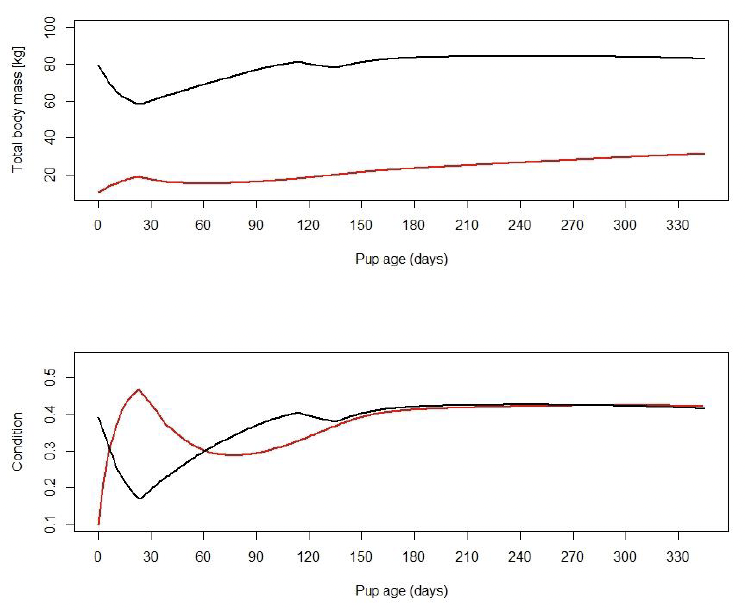
These values result in female body condition declining to around 0.15 at the end of lactation, which would suggest a value of 0.1 for ρs (Figure 9).
Relative cost of maintaining reserves (ΘF): We were unable to find any published data that would allow a value specific to harbour seals to be calculated for this parameter. We therefore used the value of 0.2 assumed by Hin et al. (2019).
Structural length and mass (K, L0, L∞, ω1, ω2, k, xo): The model developed by Hin et al. (2019) assumes that growth in length and core mass continues unabated, regardless of energy intake. This is clearly not the case in harbour seals. For example, the weight-at-age of yearling harbour seals is highly variable (Hall et al. 2012), presumably as a result of variations in foraging success among individuals. We therefore assumed that growth in harbour seals may be reduced if energy intake is less than the combined costs of metabolism, growth, and reproductive activities (pregnancy and lactation). We modelled these circumstances using a modification of the kappa (K) rule which is a fundamental component of classic DEB models (Kooijman 2010). We assumed that an individual will allocate a proportion of the assimilated energy (It) it acquires on a particular day to growth (including growth of the foetus, because this is treated as part of the female’s core mass), up to a maximum of (1-Κ)It . If this amount of energy is less than the energy required for growth, the growth rate of the female and her foetus is reduced accordingly. The balance of the energy intake is allocated to metabolism. If this balance is insufficient to cover all of the costs of metabolism, reserves must be metabolised. Values of Κ < 0.5 indicate that growth is prioritised over metabolism. In the baseline calculation we used a value of 0.1, but we explored the implications of other values (see Sensitivity analysis – Section 5.4). Growth is assumed to cease during the lactation period and the cost of lactation is given priority over metabolism.
One consequence of this approach to modelling growth is that pregnant females who experience reduced energy intake may give birth to smaller pups than those that are able to meet their total energy requirements every day.
Growth was modelled with the modified Von Bertalanffy growth curve fitted to 659 harbours seals by Hall et al. (2019)

where a is age in days, k = 0.441/365, and x0 = (- 2.02 x 365). The estimated size at birth (L0) from this equation is 82.8 cm, as also observed by Härkönen and Heide-Jørgensen (1990).
We modelled foetal growth in terms of TP and L0 as:

Where af is foetal age in days.
The relationship between structural length and structural mass for harbour seals was modelled using and , close to values estimated by Härkönen and Heide-Jørgensen (1990). We had to decrease in order to get mass at birth similar to observed values, because the masses used by Härkönen and Heide-Jørgensen (1990) included some reserve tissue. With L0 = 82.8 cm, the estimated mass at birth is 10.8 kg. There is very little information on pup mass at birth for the North Sea population. Härkönen and Heide-Jørgensen (1990) reported a range of 7.9 - 9.5 kg, which is slightly lower than our estimate, but our estimate is within the range observed for other populations (means 10.5 – 11.6 kg, Jørgensen et al. 2001, Bowen et al. 1992, 2001). Decreasing ω2 further resulted in a maximum structural mass of females that was too low. With the current values, maximum structural mass is 49.3 kg, which results in total mass of 87 kg for post-partum females, which is in the middle of the observed range of 60-110 kg (Bowen et al. 1992, 1994, 2001).
5.1.4 Energetic rates
Field metabolic maintenance scalar (σM): Although there are many estimates of the metabolic rate of harbour seals in captivity, we were unable to locate any field estimates. We used σM = 2.3. Other values were explored in the sensitivity analysis.
Energetic cost per unit structural mass (σG): We calculated growth efficiency using the same approach as Hin et al. (2019) and an energy density for foetal tissue of 6.5 MJ/kg (the mean of the values for new-born harp and harbour seal pups reported by Worthy and Lavigne(1987)). This produced a value of 25 MJ/kg for σG.
Catabolic and anabolic efficiency of reserve conversion (ε-, ε+): We used the same values as for grey seals because there was no information for these two parameters for harbour seals. See the corresponding section for grey seals for further details
Steepness of assimilation response (η): We were unable to find any data in the literature that could be used to set a feasible range for this parameter. We explored the implications of values between 5 and 40 and found that mean reproductive success was maximized when η = 20.
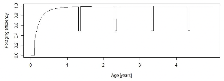
Effect of age on resource foraging efficiency (Υ, TR, pw_fast, moult_reduction, moult_duration ): Harbour pups undertake a post-weaning fast of approximately 15 days (pw_fast) (Muelbert and Bowen 1993) and continue to lose weight after this time. They regain their initial weight at weaning around the age of 5-6 months (Harding et al. 2005). We set TR = 65 days and Υ = 1.8 and assumed that foraging efficiency was 0 up to the age of 38 days (TL + pw_fast). We chose a combination of TR and Υ which resulted in a foraging efficiency of 0.95 at 1 year of age. This is considerably earlier than the foraging efficiency at this age predicted in the grey seal model because harbour seals pups accompany their mothers into the water during the lactation period, and pups have been observed catching fish at that time (Jørgensen et al. 2001).
To take account of the fact that moulting seals spend more time hauled out (Paterson et al., 2012), and are therefore likely to acquire less energy, we reduced foraging efficiency by 50% for 10 days before and after implantation (moult_duration). Figure 10 shows the modelled variation in foraging efficiency over the first 5 years of life.
5.1.5 Pregnancy
Pregnancy threshold (decision_day, skipping_point):
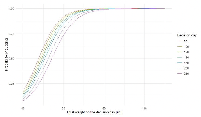
To our knowledge, there is no information for harbour seals equivalent to that for grey seals on the relationship between a female’s mass at the end of lactation and the likelihood of giving birth in the following breeding season. Unlike grey seals, harbour seals also forage regularly during lactation and increase their mass from the end of lactation until implantation (e.g., Renouf et al. 1991). We therefore estimated the combination of decision_day and weight at weaning that results in a 50% probability of giving birth in the next year (skipping_point), which resulted in most mature females (age > = 4) becoming pregnant every year. The interpretation of this point is not equivalent to this interpretation for grey seals due to different breeding strategies of these two species.
We also looked at whether our parameter choice resulted in the probability of giving birth being close to one for females which weigh 60 kg at the last day of pregnancy– the lowest weight reported for harbour seal females just before giving birth (Bowen et al. 2001, Figure 11). For the final simulations, we used decision_day – 160 (as for grey seals) and skipping_point = 45 kg. See sensitivity analysis for further analysis.
5.1.6 Lactation
Efficiency of conversion of mother's reserves to pup tissue (σL): Lang et al. (2011) estimated that approximately 70% of the energy obtained by grey seal pups from milk was converted into tissue. However, this “storage efficiency” includes the costs of maintenance. We, therefore, used the value of 0.86 from Hin et al (2019), as for the grey seal model.
Effect of pup age on milk assimilation (TC,, lact_feed, R_prop_lactation): The reproductive strategy of harbour seals is intermediate between capital and income breeding, because females start foraging before the end of lactation. We, therefore, modelled a 10% decrease in milk provisioning by female at Tc = 0.70 * TL (equivalent to day 16 of lactation) and assumed that females start foraging at lact_feed = 10 days with a foraging efficiency of 0.6 (R_prop_lactation). These days correspond to values reported by Boness et al (1994); Thompson et al (1994), and Bowen et al (2001). There is little information, however, on the amount of food females obtain during lactation, and various values of R_prop_lactation were therefore explored (see Sensitivity analysis).
Effect of female body condition on milk assimilation (ξM): the value of ξM had little effect on model results (not presented in this report) and we chose value 2.
Lactation scalar (ΦL ,pup_mass_gain, daily_pup_ee, ε, ρpup). All of a pup’s energy requirements during the lactation period must be supplied by milk. Although harbour seal pups are reported to start foraging before weaning, it applies to small number of individuals and is more common in pups that have a long lactation period (Jørgensen et al. 2001, Sauvé et al. 2014). There is no information on energy expenditure of harbour seal pups. We used calculation by Reilly et al. (1996) estimating that grey seal pups expend 13.5 MJ/day during lactation, corresponding to 3.7 * RMR and, therefore, resulting in daily_pup_ee = 8.3 MJ/day for a 15 kg harbour seal pup. (Bowen et al. 1992, Dubé et al. 2003, Muelbert et al. 2003, Sauvé et al. 2014) reported daily mass increase of harbour seal pup to be between 0.40 and 0.80 kg/day. Assuming the estimated mass at birth to be 10.8 kg and TL = 23, values of pup_mass_gain = 0.55 kg/day would result in simulated mass at weaning of 23.45 kg, as observed (Muelbert et al. 2003, Jørgensen et al. 2001) Assuming that mass at birth is entirely composed of structural mass, this implies that a pup’s body condition at the end of lactation is 0.5. Using this value in Hin et al.’s (2019) formula gives ΦL = 4.51 if ε = 25.8 MJ/kg.
5.1.7 Mortality
Age-dependent mortality rate (max_age, α1, α2, β1, β2): We followed Hin et al. (2019) and estimated changes in the probability of survival with age using the approach developed by Barlow & Boveng (1991). The following function describing the variation in daily survival with age:

where a is age in days, was fitted to the annual age-specific harbour seal survival rates documented in Sinclair et al. (2020). We used values for a stable population (e.g., Moray Firth, Table 13 of Sinclair et al. 2020) in order to investigate the effects of disturbance on a population that is not food-limited, and for a population increasing at 3-4% per annum using the demographic rates suggested in Table 16 of Sinclair et al. (2020). In the latter case Rmean was then adjusted to 1.61 so that the population growth rate was 1.00 to investigate the effects of disturbance on a population that was food-limited. Figure 12 shows the resulting relationship between age and cumulative survival, with maximum age of 30 years (max_age) and
α1 = 0.0022
β1 = 0.0019
α2 = 0.00021
β2 = 0.0000003
for a stable population and:
α1 = 0.005
β1 = 0.0055
α2 = 0.00013
β2 = 0.0000000036
for an increasing population.
The life expectancy of each simulated female was calculated by choosing a random number between 0 and 1 and determining the age in days at which cumulative survival equalled this value.

We also assumed that there was some mortality of foetuses during pregnancy. In the baseline model mortality over the entire duration of the pregnancy was set at foetal_mortality = 0.1.
Starvation-induced mortality rate (μs): No empirical information that could provide a species-specific value of this parameter for harbour seals is available. We used the value of 0.2 proposed by Hin et al. (2019) and used for grey seal DEB.
5.2 Model results – pattern-oriented modelling
The following results are based on 50 simulations for 1000 females each.
5.2.1 Annual changes in mother and pup condition and total body weight
Total body weight and condition of the modelled females are at maximum at the start of lactation and at a minimum at the end of lactation. They increase soon after lactation, as described by Renouf et al. (1993). Bowen et al. (2001) documented that during the initial 80% of lactation, females lose 32.3% of their postpartum body mass and their mean reserve mass at parturition is 43% of the total body mass, which is also the case for the modelled females (Figure 9).
Pup condition is at maximum of around 0.43 at the end of lactation, which corresponds to values reported by Muelbert et al. (2003). The total weight of a pup at 1 year of age is approximately 31 kg, which also corresponds to values reported by Muelbert et al. (2003). The simulated weight of a pup at around 110 days (17 kg) is slightly lower than the 20-30 kg observed by Harding et al. (2005). Two months later simulated total weight is around 23 kg, within the range reported by Harding et al. (2005) (Figure 9 & Figure 13).
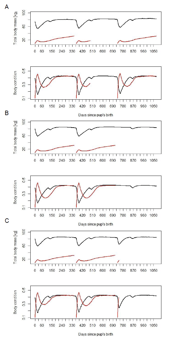
Figure 13 shows examples from three different females whose body mass and condition are displayed for three consecutive years. Panel A shows a female who gave birth in three consecutive years; panel B shows a female who skips the third pregnancy; and panel C shows a female whose pup dies before weaning. The body mass and condition of this female return to the pre-parturition level more quickly than for females that nurse their pups until weaning.
5.2.2 Birth rate: proportion of adult females breeding
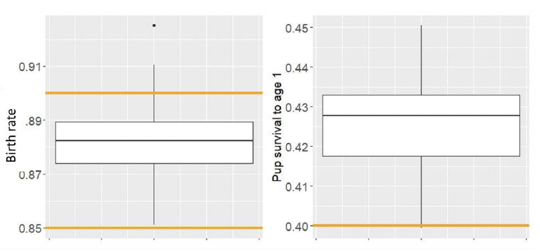
The proportion of adult females giving birth to a pup each year (birth rate) showed little variation between simulations and was within the range observed in the wild populations (Figure 14).
5.2.3 Pup survival to age 1
Pup survival to age 1 showed relatively large variation between simulations. It was higher than the value recommended by Sinclair et al. (2020) for stable population (Figure 14).
5.3 Simulating the effect of disturbance
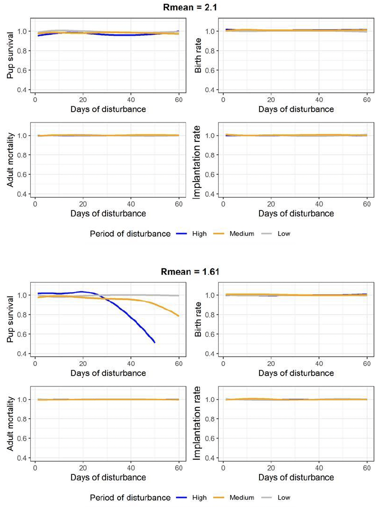
Disturbance was modelled by reducing energy intake by 16% on each day of disturbance. This is based on studies by (Russell et al. 2016) which showed that although seals are displaced from an area when piling occurs, they return within two hours after piling stops. Given the average piling duration is 6 hours, this implies that seals are displaced from an area for 8 hours. We assumed that they can still forage at 50% of the normal rate while they are displaced. This results in the loss of 4 hours of foraging time (16% of the day). We modelled the effect of 1, 2, 3, 4, 5, 7, 10, 15, 20, 25, 30, 40, 50, and 60 days of disturbance and simulated 4500 11 and 21 year-old females for two values of Rmean: Rmean = 2.1 for a population that is not limited by food, and Rmean = 1.61 for a population that is food-limited (see Section 5.1.7). We chose 11 and 21 years-old females to understand the difference between younger females which may express higher costs of pregnancy. We modelled disturbance scenarios at three different life history stages of females and pups: i) low impact: disturbance happens from implantation day to the day on which a female decides whether or not to continue with pregnancy (a period of approximately 5 months); ii) medium impact: disturbance occurs between the decision day and parturition (a period of approximately 3 months); iii) high impact: disturbance occurs between giving birth and implantation (a period of approximately 4 months). Figure 15 shows these three periods in relation to changes in female body condition. The days on which disturbance occurred within each period were chosen at random.

We analysed the effect of disturbance on four vital rates over the course of the year when the disturbance happened: pup survival to age 1, adult mortality, birth rate, and implantation rate.
There was no difference in the effect of disturbance between 11- and 21-years old females. The disturbance had no effect on any of the four vital rates regardless of the duration of disturbance or the disturbance period when food is not a limiting factor (Figure 16, top four panels). When food is a limiting factor, disturbance had the highest effect on pup survival and this effect was most pronounced for the ‘High impact’ disturbance period. The remaining three vital rates were not affected regardless of the duration of disturbance or the disturbance period (Figure 16, bottom four panels).
5.4 Sensitivity analysis
The aim of the sensitivity analysis (SA) was to explore the influence of parameter values outside the ranges used in the model simulation on the outputs of the model. SA is frequently based on parameters which either have a large range reported in literature or arbitrary parameters which cannot be directly measured. From the list of all parameters, we tested the effect of varying K, Tr, σM, decision_day and R_prop_lactation (Table 5). We also tested the effect of mu_s and upsilon and results can be presented on demand. Although, there are other parameters used in the model which either have a large range reported in literature or arbitrary parameters which cannot be directly measured, we chose the ones which were not already used in the design phase of model (such as η) or parameters, which were directly copied from other species, due to no information in the literature specific for harbour seals (like ε-, ε+, ΘF)
| Name of parameter | Description | Value used in the final model simulation | Variation range in the sensitivity analysis |
|---|---|---|---|
| K | Proportion of assimilated energy allocated to growth when energy intake is limited | 0.1 | ± 0.1 |
| TR | Age at which calf’s resource foraging efficiency is 50% | 65 days | ± 20 days |
| σM (sigma_m) | Field metabolic maintenance scalar | 2.3 | ± 0.2 |
| decision_day | Day of pregnancy when female decides whether or not to continue | 160 days | ± 40 days |
| R_prop_lactation | Foraging efficiency during lactation | 0.6 | ± 0.2 |
We analysed both the effect of varying one parameter at a time and the interaction between them by varying parameters simultaneously. We followed the Design of Experiment methodology first formulated by (Lorscheid et al. 2012) and applied to individual based models (IBMs) by Thiele et al. (2014). We used a full factorial design of the extreme values of each of the parameters (Table 5), leading to 32 combinations, and we ran one simulation for 500 females for each of these combinations. We then analysed the results using the FrF2 (Groemping 2011) and DoE.base (Groemping 2013) packages in R, following the description by Thiele et al. (2014). We did not run stepwise fitting of a linear regression model to the SA data, as suggested by Thiele et al. (2014), but we based our conclusions on visual analysis of the plots, as discussed below. The results of regression models can be strongly influenced by the sample size, and do not necessarily reflect the actual effect of different parameters (White et al. 2014).
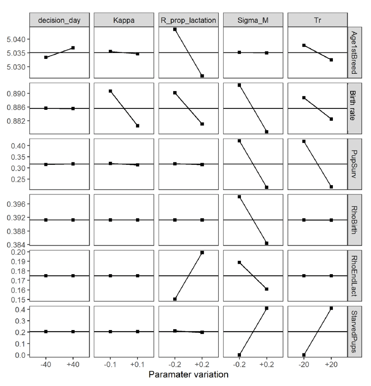
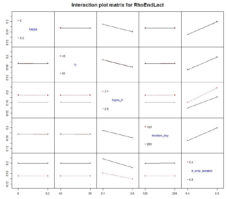
We used the following patterns in SA: mean age of first breeding (Age1stBreed), mean proportion of adult females breeding (Fertility), mean reproduction success defined as proportion of pups which survived to age 1 (PupSurv), mean female condition at parturition (RhoBirth), mean female condition at the end of lactation (RhoEndLact) and mean number of pups which died of starvation (StarvedPups).
5.4.1 Main effect: varying one parameter at the time
The chosen parameters had very little effect on Age1stBreed, Fertility, RhoBirth: these patterns varied little during SA. Sigma_M has the largest effect on the remaining patterns; increasing in Tr resulted in increased pup mortality due to starvation and reducing R_prop_lactation from 0.6 to 0.2 resulted in a decline in RhoEndLact from 0.175 to 0.15 (Figure 17). (Hall et al., 2019)
5.4.2 Interaction effect: varying two parameters at the time
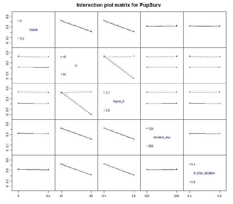
Simultaneous increase in Sigma_M and Tr resulted in large increase in the number of pups that died from starvation. The reduction in RhoEndLact was larger when females foraged little during lactation than when only energy expenditure (Sigma_M) was increased (Figure 18). Varying remaining combinations of parameters had little effect on model results.
Contact
Email: ScotMER@gov.scot
There is a problem
Thanks for your feedback