Gender export gap in Scotland: research
Research commissioned by the Scottish Government to understand what is holding women back from exporting and the difference their increased participation in trade could make to Scotland’s economy.
Appendix 6: Methodological note
We used a conditional difference-in-difference (CDiD) approach which combines propensity score matching (PSM) and difference-in-difference (DiD) approaches to identify the direct impacts of entering an export market. The CDiD approach is a two-step process that allowed us to estimate the difference between turnover and number of employees before and after SME entry into an export market. This approach is frequently used for policy evaluation and recommended in HM Treasury’s Magenta Book[8].
However, there are several limitations which need to be accounted for:
1) There is a conditional independence assumption which assumes that the observable differences between the treated (exporters) and non-treated (non-exporters) group can be controlled and therefore the outcome that would occur in the absence of treatment would be the same in both cases.
2) The approach requires a rich dataset that contains the key variables that affect both the decision to enter export markets, appropriate outcome variables, and appropriate control variables. The LSBS contains a rich number of variables to be able to conduct this analysis, however, when looking at Scotland, the number of observations in a sub-sample becomes quite low.
3) The matching procedure cannot account for unobservable characteristics that can interact with the measured outcomes (e.g., managerial characteristics). Even though the LSBS contains a vast number of variables we are limited by the sample size in what we can apply.
4) When sample sizes for either control or treatment groups are small, as is the case for women-led exporters in Scotland, estimations run the risk of yielding imprecise estimates.
Despite these limitations the results are still valid as we took several steps to ensure the robustness of our analysis. Our starting point for the conditional difference-in-difference analysis was all SMEs in the UK. From here we selected firms that exported in 2018 and discarded firms that exported before 2018. We also discarded any company that says they do not know if they exported or did not export. Our treatment groups are therefore SMEs that exported in 2018 while the control group were the non-exporters.
Both groups were then split into two: observations for the whole UK, and observations for Scotland only. The remaining number of single treated firms in the UK is 3,333 and in Scotland is 182. While the number of potential control UK firms in the 2017-2020 period ranges from 5143 up to 11,579, the number of potential control Scottish firms in the 2017-2020 period ranges from 547 up to 903.
To aid further analysis and fulfil the objective of this study, these groups were further divided into two: women/equally led SMEs and male-led SMEs. The single treated women/equally led SMEs in the UK is 1,579 and in Scotland is 52. While the single treated male-led SMEs in the UK is 3128 and in Scotland is 100. For the potential control women/equally led SMEs in the UK, the number in the 2017-2020 period ranges from 1,809 up to 4,842, and in Scotland ranges from 206 to 343. For the male-led SMEs in the UK, the number of the potential control ranges between 3084 to 6288, and in Scotland, it ranges between 368 and 487.
Our outcome variable was the average turnover and number of employees. The main identification challenge for estimation purpose is to know what would have happened with the firms exporting had they not started exporting. It is important we find a control group of firms similar to those who are exporting, because those who are exporting might differ systematically from the firm who are not exporting. The key identifying assumption behind this procedure is that the treated group’s outcome variables would behave like the control group’s outcomes if there were no exportation.
For the impact analysis, we employ the difference-in-differences (DiD) matching estimator. This approach enables us to compare the changes in firm performance between exporting firms (treatment group, T) and their matched non-exporting counterparts (control group, NT). Let YTj,t represent the logarithm of the outcome measure 𝑌 for treated firm j in year t. The difference in the log of the outcome measure between year t and 𝑡−1 for treated firm j is defined as ΔYTj,t = YTj,t – YTj,t − 1. The same quantities are computed for the firms in the control group (NT). We then obtain the average treatment effect on the treated (ATET) by comparing these differences. The ATET is calculated as follows:
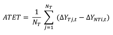
Where 𝑁𝑇 is the number of treated firms, and 𝑌𝑇𝑗,t and Δ𝑌𝑁𝑇𝑖,𝑡 are the log differences for treated and matched control firms, respectively. In the matching procedure, all variables related to the treatment assignment and the outcome were included. Each treated firm is matched with a control firm considering performance measures and observable characteristics in the before-treatment period. As matching using the exact values of all covariates is not possible, treated firms and control firms are matched using the propensity score estimated via a logistic regression model with a set of pre-treatment attributes. This method estimates the conditional probability that a firm exports based on firm characteristics.
We selected three sets of independent variables for our matching approach: location type as urban or rural, industry sector[9], and geographical context as England, Scotland, Wales and Northern Ireland. Our goal is to identify the most similar control firm for each treated firm based on these variables to accurately estimate the propensity score. Given this objective, we are not concerned with multicollinearity among the variables, as we do not interpret the probit regression coefficients or their standard errors. Instead, we focus on the propensity score, i.e., the overall fit of the logistic regression, and more importantly, on achieving covariate balance after matching.
With the estimated propensity score, we conduct Kernel matching, matching each treated unit with multiple control units with different weights. There was 1,579 treated women/equally led SMEs in the UK. As all the firms were matched during the Kernel matching, the final number of treated firms remains 1,579 while the control firms are 9,022.
For the male-led SMEs in the UK, no treated firms were eliminated as there were matching control firms. The final number of treated firms is 3,128 while the matching approach identified 8,994 control firms.
None of the 52 treated women/equally led SMEs in Scotland were eliminated because they all had matching control firms. The final number of control firms is 610. Of the 100 treated male-led SMEs in Scotland, none were eliminated. The final number of untreated firms was 824.
After matching, we performed the DiD analysis to estimate the treatment effect. This involved three steps. Firstly, we calculated the difference in the outcome variable before and after the treatment period.
For treated firms (T):
ΔYTj,t = YTj,t – YTj,t-1
For matched control firms (NT):
ΔYNTi,t = YNTi,t – YNTi,t-1
Then we computed the difference between the changes in outcome for treated and control firms: Di = ΔYTj,t – ΔYNTi,t. Finally, we calculated the average of these differences to estimate the ATET. The weighted difference in difference is then:
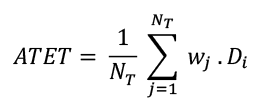
Where wj are the weights assigned to the matched control units, NT is the number of treated units, and 𝐷j is the DiD for treated unit j.
Results
Tables A1 – A4 present the results from the PSM and DiD for Women-led and equally led SMEs Scotland.
Tables A5 – A8 present the results from the PSM and DiD for male-led SMEs Scotland
Tables A9 – A12 present the results from the PSM and DiD for women-led and equally-led SMEs UK
Tables A13 – A16 present the results from the PSM and DID for male-led SMEs UK
Table A1: Propensity Score Matching – Kernel – Women-led and equally led SMEs Scotland
Logistic regression
Log likelihood = -177.15655
Number of obs = 662
LR chi2(2) = 10.07
Prob > chi2 = 0.0065
Pseudo R2 = 0.0276
| Treatment | Coefficient | Std. err. | z | P>|z| | [95% conf. interval] | [95% conf. interval] |
|---|---|---|---|---|---|---|
| SIC1DIG | -.1312139 | .0433824 | -3.02 | 0.002 | -.2162418 | -.0461861 |
| URBRUR1 | -.0135541 | .0430281 | -0.32 | 0.753 | -.0978876 | .0707794 |
| _cons | -1.445121 | .7010589 | -2.06 | 0.039 | -2.819172 | -.0710711 |
Table A2: PSTest – Kernel – Women-led and equally led SMEs Scotland
Verification that the covariates are balanced across treated and control groups after matching.
| Variable | Treated | Control | %bias | t | p>|t| | V(C) |
|---|---|---|---|---|---|---|
| SIC1DIG | 5.3846 | 5.9175 | -14.5 | -0.76 | 0.449 | 1.19 |
| URBRUR1 | 15.154 | 15.246 | -2.8 | -0.14 | 0.889 | 0.98 |
* if variance ratio outside [0.57; 1.74]
| Ps R2 | LR chi2 | p>chi2 | MeanBias | MedBias | B | R | %Var |
|---|---|---|---|---|---|---|---|
| 0.004 | 0.61 | 0.736 | 8.6 | 8.6 | 15.2 | 1.15 | 0 |
* if B>25%, R outside [0.5; 2]
| P1_2018 | Coefficient | Std. err. | t | P>|t| | [95% conf. interval] | [95% conf. interval] |
|---|---|---|---|---|---|---|
| Treatment | -599156.3 | 1298234 | -0.46 | 0.645 | -3153525 | 1955212 |
| Time | 364459.8 | 383998.2 | 0.95 | 0.343 | -391084.3 | 1120004 |
| DiD | 2217040 | 1504154 | 1.47 | 0.142 | -742491.9 | 5176572 |
| _cons | 677322.9 | 314868 | 2.15 | 0.032 | 57797.52 | 1296848 |
Number of obs = 317
| P1_2019 | Coefficient | Std. err. | t | P>|t| | [95% conf. interval] | [95% conf. interval] | |
|---|---|---|---|---|---|---|---|
| Treatment | -599156.3 | 825968.5 | -0.73 | 0.469 | -2227232 | 1028920 | |
| Time | 473150.8 | 275927.6 | 1.71 | 0.088 | -70733.18 | 1017035 | |
| DiD | 3672016 | 1070650 | 3.43 | 0.001 | 1561646 | 5782386 | |
| _cons | 677322.9 | 200326.8 | 3.38 | 0.001 | 282456.5 | 1072189 | |
Number of obs = 218
| P1_2018 | Coefficient | Std. err. | t | P>|t| | [95% conf. interval] | [95% conf. interval] | |
|---|---|---|---|---|---|---|---|
| Treatment | -13.67521 | 9.240045 | -1.48 | 0.140 | 31.83124 | 4.480818 | |
| Time | 2.687264 | 2.724976 | 0.99 | 0.325 | -2.66712 | 8.041647 | |
| DiD | 10.29564 | 10.74955 | 0.96 | 0.339 | -10.82645 | 31.41774 | |
| _cons | 14.23077 | 2.2484 | 6.33 | 0.000 | 9.812823 | 18.64872 | |
Number of obs = 483
| P1_2019 | Coefficient | Std. err. | t | P>|t| | [95% conf. interval] | [95% conf. interval] | |
|---|---|---|---|---|---|---|---|
| Treatment | -13.67521 | 10.44262 | -1.31 | 0.191 | -34.22208 | 6.871653 | |
| Time | 4.691309 | 3.528799 | 1.33 | 0.185 | -2.251943 | 11.63456 | |
| DiD | 4.353136 | 14.40057 | 0.30 | 0.763 | -23.98137 | 32.68764 | |
| _cons | 14.23077 | 2.541026 | 5.60 | 0.000 | 9.231056 | 19.23048 | |
Number of obs = 316
Table A5: Propensity Score Matching – Kernel – male-led SMEs Scotland
Logistic regression
Log likelihood = -315.67629
Number of obs = 924
LR chi2(2) = 2.12
Prob > chi2 = 0.3464
Pseudo R2 = 0.0033
| Treatment | Coefficient | Std. err. | z | P>|z| | [95% conf. interval] | [95% conf. interval] |
|---|---|---|---|---|---|---|
| SIC1DIG | -.01039 | .0303715 | -0.34 | 0.732 | -.0699171 | .0491371 |
| URBRUR1 | .0486051 | .0342882 | 1.42 | 0.156 | -.0185985 | .1158088 |
| _cons | -2.78052 | .5666454 | -4.91 | 0.000 | -3.891125 | -1.669916 |
Table A6: PSTest – Kernel – male-led SMEs Scotland
Verification that the covariates are balanced across treated and control groups after matching.
Mean t-test V(T)/
| Variable | Treated | Control | %bias | t | p>|t| | V(C) |
|---|---|---|---|---|---|---|
| SIC1DIG | 5.7 | 5.8581 | -4.5 | -0.32 | 0.752 | 1.00 |
| URBRUR1 | 15.28 | 14.734 | 18.8 | 1.37 | 0.173 | 0.99 |
* if variance ratio outside [0.67; 1.49]
| Ps R2 | LR chi2 | p>chi2 | MeanBias | MedBias | B | R | %Var |
|---|---|---|---|---|---|---|---|
| 0.007 | 1.90 | 0.387 | 11.6 | 11.6 | 19.5 | 1.06 | 0 |
* if B>25%, R outside [0.5; 2]
| P1_2018 | Coefficient | Std. err. | t | P>|t| | [95% conf. interval] | [95% conf. interval] |
|---|---|---|---|---|---|---|
| Treatment | 1155691 | 2216199 | 0.52 | 0.602 | -3202044 | 5513426 |
| Time | 1133489 | 572875.2 | 1.98 | 0.049 | 7038.806 | 2259940 |
| DiD | 4832569 | 2508313 | 1.93 | 0.055 | -99551.9 | 9764689 |
| _cons | 772642.5 | 426507.7 | 1.81 | 0.071 | -66004 | 1611289 |
Number of obs = 517
| P1_2019 | Coefficient | Std. err. | t | P>|t| | [95% conf. interval] | [95% conf. interval] |
|---|---|---|---|---|---|---|
| Treatment | 1155691 | 1727205 | 0.67 | 0.504 | -2243956 | 4555337 |
| Time | 416978.2 | 514186.3 | 0.81 | 0.418 | -595091.2 | 1429047 |
| DiD | 4777001 | 2052904 | 2.33 | 0.021 | 736283.5 | 8817719 |
| _cons | 772642.5 | 332400.8 | 2.32 | 0.021 | 118380.2 | 1426905 |
Number of obs = 379
| P1_2018 | Coefficient | Std. err. | t | P>|t| | [95% conf. interval] | [95% conf. interval] |
|---|---|---|---|---|---|---|
| Treatment | -.8320921 | 16.80546 | -0.05 | 0.961 | -33.82926 | 32.16508 |
| Time | 3.154385 | 3.70311 | 0.85 | 0.395 | -4.116594 | 10.42536 |
| DiD | 32.91704 | 18.03711 | 1.82 | 0.068 | -2.49846 | 68.33255 |
| _cons | 16.26066 | 3.011419 | 5.40 | 0.000 | 10.3478 | 22.17352 |
Number of obs = 680
| P1_2019 | Coefficient | Std. err. | t | P>|t| | [95% conf. interval] | [95% conf. interval] |
|---|---|---|---|---|---|---|
| Treatment | -.8320921 | 19.25117 | -0.04 | 0.966 | -38.66048 | 36.9963 |
| Time | 3.872957 | 4.766896 | 0.81 | 0.417 | -5.493956 | 13.23987 |
| DiD | 36.3281 | 21.78138 | 1.67 | 0.096 | -6.472143 | 79.12834 |
| _cons | 16.26066 | 3.449672 | 4.71 | 0.000 | 9.482085 | 23.03924 |
Number of obs = 477
Table A9: Propensity Score Matching – Kernel – women-led and equally-led SMEs UK
Logistic regression
Log likelihood = -4355.2693
Number of obs = 10,601
LR chi2(2) = 212.97
Prob > chi2 = 0.0000
Pseudo R2 = 0.0239
| Treatment | Coefficient | Std. err. | z | P>|z| | [95% conf. interval] | [95% conf. interval] |
|---|---|---|---|---|---|---|
| SIC1DIG | -.1073064 | .0078465 | -13.68 | 0.000 | -.1226851 | -.0919276 |
| -.3283033 | .0625253 | -5.25 | 0.000 | -.4508507 | -.205756 | |
| URBRUR1 | .0291547 | .0078677 | 3.71 | 0.000 | .0137342 | .0445752 |
| _cons | -.8432934 | .080438 | -10.48 | 0.000 | -1.000949 | -.6856377 |
Table A10: PSTest – Kernel – women-led and equally-led SMEs UK
Verification that the covariates are balanced across treated and control groups after matching.
Mean t-test V(T)/
| Variable | Treated | Control | %bias | t | p>|t| | V(C) |
|---|---|---|---|---|---|---|
| SIC1DIG | 6.0431 | 6.3827 | -9.7 | -2.85 | 0.004 | 0.88* |
| 1.1951 | 1.1982 | -0.5 | -0.14 | 0.888 | 1.18* | |
| URBRUR1 | 7.5624 | 7.5515 | 0.2 | 0.06 | 0.950 | 1.03 |
* if variance ratio outside [0.91; 1.10]
| Ps R2 | LR chi2 | p>chi2 | MeanBias | MedBias | B | R | %Var |
|---|---|---|---|---|---|---|---|
| 0.002 | 8.57 | 0.036 | 3.5 | 0.5 | 10.4 | 0.92 | 67 |
* if B>25%, R outside [0.5; 2]
| P1_2018 | Coefficient | Std. err. | t | P>|t| | [95% conf. interval] | [95% conf. interval] |
|---|---|---|---|---|---|---|
| Treatment | 2224494 | 907644.4 | 2.45 | 0.014 | 445020.2 | 4003968 |
| Time | 33469.96 | 190583.5 | 0.18 | 0.861 | -340176.8 | 407116.8 |
| DiD | -433432.4 | 930919.1 | -0.47 | 0.642 | -2258538 | 1391673 |
| _cons | 1199266 | 171406.3 | 7.00 | 0.000 | 863216.6 | 1535315 |
Number of obs = 4,116
| P1_2019 | Coefficient | Std. err. | t | P>|t| | [95% conf. interval] | [95% conf. interval] |
|---|---|---|---|---|---|---|
| Treatment | 2200484 | 961394.2 | 2.29 | 0.022 | 315235.5 | 4085733 |
| Time | 225596.9 | 216523.8 | 1.04 | 0.298 | -198996.2 | 650189.9 |
| DiD | -709177 | 1006149 | -0.70 | 0.481 | -2682188 | 1263834 |
| _cons | 1199266 | 178015.6 | 6.74 | 0.000 | 850185.4 | 1548346 |
Number of obs = 2,404
| P1_2018 | Coefficient | Std. err. | t | P>|t| | [95% conf. interval] | [95% conf. interval] |
|---|---|---|---|---|---|---|
| Treatment | 5.722589 | 5.713455 | 1.00 | 0.317 | -5.477737 | 16.92291 |
| Time | -1.518149 | 1.151324 | -1.32 | 0.187 | -3.775139 | .7388398 |
| DiD | -3.372967 | 5.847555 | -0.58 | 0.564 | -14.83617 | 8.090239 |
| _cons | 17.58044 | 1.046305 | 16.80 | 0.000 | 15.52933 | 19.63156 |
Number of obs = 6,284
| P1_2019 | Coefficient | Std. err. | t | P>|t| | [95% conf. interval] | [95% conf. interval] |
|---|---|---|---|---|---|---|
| Treatment | 5.982058 | 6.241971 | 0.96 | 0.338 | -6.256442 | 18.22056 |
| Time | -.7554416 | 1.372502 | -0.55 | 0.582 | -3.446478 | 1.935594 |
| DiD | -5.133374 | 6.538488 | -0.79 | 0.432 | -17.95325 | 7.686502 |
| _cons | 17.58044 | 1.126211 | 15.61 | 0.000 | 15.3723 | 19.78858 |
Number of obs = 3,323
Table A13: Propensity Score Matching – Kernel – male-led SMEs UK
Logistic regression
Log likelihood = -6829.5756
Number of obs = 12,120
LR chi2(2) = 182.98
Prob > chi2 = 0.0000
Pseudo R2 = 0.0132
| Treatment | Coefficient | Std. err. | z | P>|z| | [95% conf. interval] | [95% conf. interval] |
|---|---|---|---|---|---|---|
| SIC1DIG | -.0758681 | .006262 | -12.12 | 0.000 | -.0881414 | -.0635948 |
| NATION | -.2832519 | .0458586 | -6.18 | 0.000 | -.3731332 | -.1933707 |
| URBRUR1 | .0350445 | .0061208 | 5.73 | 0.000 | .023048 | .047041 |
| _cons | -.5249238 | .0584706 | -8.98 | 0.000 | -.6395242 | -.4103235 |
Table A14: PSTest – Kernel – male-led SMEs UK
Verification that the covariates are balanced across treated and control groups after matching.
Mean t-test V(T)/
| Variable | Treated | Control | %bias | t | p>|t| | V(C) |
|---|---|---|---|---|---|---|
| SIC1DIG | 5.6202 | 5.7688 | -4.4 | -1.84 | 0.065 | 0.99 |
| NATION | 1.2276 | 1.2154 | 1.7 | 0.71 | 0.478 | 1.24* |
| URBRUR1 | 8.0531 | 7.9378 | 2.3 | 0.89 | 0.371 | 1.09* |
* if variance ratio outside [0.93; 1.07]
| Ps R2 | LR chi2 | p>chi2 | MeanBias | MedBias | B | R | %Var |
|---|---|---|---|---|---|---|---|
| 0.000 | 4.31 | 0.230 | 2.8 | 2.3 | 5.2 | 1.04 | 67 |
*if B>25%, R outside [0.5; 2]
| P1_2018 | Coefficient | Std. err. | t | P>|t| | [95% conf. interval] | [95% conf. interval] |
|---|---|---|---|---|---|---|
| Treatment | 494906.3 | 1385753 | 0.36 | 0.721 | -2221761 | 3211574 |
| Time | 684292.3 | 313659.2 | 2.18 | 0.029 | 69386.25 | 1299198 |
| DiD | 2988281 | 1409905 | 2.12 | 0.034 | 224266.6 | 5752296 |
| _cons | 1575687 | 282314.8 | 5.58 | 0.000 | 1022230 | 2129145 |
Number of obs = 5,130
| P1_2019 | Coefficient | Std. err. | t | P>|t| | [95% conf. interval] | [95% conf. interval] |
|---|---|---|---|---|---|---|
| Treatment | 494906.3 | 1612836 | 0.31 | 0.759 | -2667513 | 3657326 |
| Time | 542184.3 | 399883.1 | 1.36 | 0.175 | -241899.4 | 1326268 |
| DiD | 2650130 | 1669312 | 1.59 | 0.112 | -623026.9 | 5923287 |
| _cons | 1575687 | 328577.6 | 4.80 | 0.000 | 931418.3 | 2219957 |
Number of obs = 2,905
| P1_2018 | Coefficient | Std. err. | t | P>|t| | [95% conf. interval] | [95% conf. interval] |
|---|---|---|---|---|---|---|
| Treatment | 1.777606 | 6.729196 | 0.26 | 0.792 | -11.41364 | 14.96885 |
| Time | .69126 | 1.441193 | 0.48 | 0.631 | -2.133911 | 3.516431 |
| DiD | 11.63924 | 6.834401 | 1.70 | 0.089 | -1.758241 | 25.03671 |
| _cons | 18.4066 | 1.307195 | 14.08 | 0.000 | 15.84411 | 20.9691 |
Number of obs = 7,067
| P1_2019 | Coefficient | Std. err. | t | P>|t| | [95% conf. interval] | [95% conf. interval] |
|---|---|---|---|---|---|---|
| Treatment | 1.777606 | 6.788228 | 0.26 | 0.793 | -11.53147 | 15.08668 |
| Time | .2383565 | 1.615442 | 0.15 | 0.883 | -2.928896 | 3.405609 |
| DiD | 7.221756 | 7.01825 | 1.03 | 0.304 | -6.5383 | 20.98181 |
| _cons | 18.4066 | 1.318662 | 13.96 | 0.000 | 15.82122 | 20.99199 |
Number of obs = 3,673
Contact
Email: monika.dybowski@gov.scot
There is a problem
Thanks for your feedback