Marine mammals: methodology for combining data

Section 3: Case Study - Estimating Harbour Porpoise Density in the Moray Firth

Various datasets were considered for the case study, yet concurrently collected DAS and PAM data in 2010 in the Moray Firth were the only data that met the project requirements to focus on (1) PAM and DAS data (2) with harbour porpoise as the target species (3) in Scotland. Therefore, this dataset became the focus of the project case study. The data were previously presented in both Thompson et al. (2013) and Williamson et al. (2016).

Data overview and previous work

Thompson et al. (2013) used an extensive deployment of 70 CPODs in 2010 to assess the response of harbour porpoise to seismic surveys, focussing on two 25 x 25 km study blocks in the Moray Firth. Williamson et al. (2016) then used the CPOD data to compare these PAM data with density estimates derived from visual-aerial surveys, and compared the visual-aerial density estimates with those derived from DAS data. The aerial surveys occurred between August and September 2010. Visual-aerial surveys were conducted on ten days during the Aug-Sept 2010 survey period, and the DAS surveys occurred on four days. The majority of CPODs were deployed between June and November 2010. The main details of the CPOD and DAS data are given in the Materials and Methods section, though further details are given in Williamson et al. (2016).

Williamson et al. (2016) compared typical CPOD data outputs e.g., detections per minute, and other coarser time resolutions, with the density estimates from both sets of aerial data. The density estimates produced from the DAS data in Williamson et al. (2016) were considered to be relative estimates as no estimate of g(0) was available from the survey data to correct for availability bias, though a parameter from Hammond et al. (2013) was applied to the visual-aerial data. Therefore, the visual-aerial data were used to estimate absolute abundance estimates. Density surface modelling using GAMs in the R package dsm (Miller et al., 2022) was conducted using the visual- and the digital-aerial data separately. Candidate environmental variables used in spatial modelling were depth, slope, sediment type (proportion of sediment that was sand or gravelly sand) and distance from the coast. The comparison of the density surfaces yielded similar patterns. Correlation was also evident between the CPOD data and corresponding absolute densities from the visual-aerial data (Williamson et al., 2016).

Materials and Methods

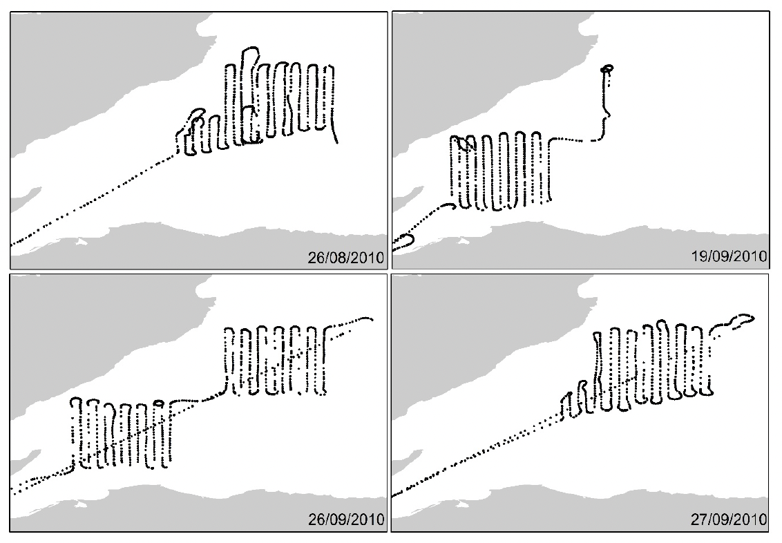
As described in Williamson et al. (2016), the DAS data were collected by HiDef Aerial Surveying Ltd on 4 days in Aug – Sept 2010 (28 Aug, 19 Sept, 26 Sept, 27 Sept) between 10:00 and 16:00 depending on the surveyed day. On each day, a randomly selected route was chosen, along planned transect lines (Fig. 3). Flight height varied between 244 and 457 m depending on cloud height, resulting in a strip width between 80 – 150 m. Detectability was assumed to be certain across the whole strip width. The effective strip half widths of the surveys were therefore between 40 – 75 m.

We used similar methods as applied in Jacobson et al. (2017), with the following workflow.

Absolute density estimation (DAS)

• Estimate a density surface using the DAS data. Jacobson et al. (2017) used Gauss-Markov smoothing to prevent over-smoothing and retain observed patchiness in harbour porpoise distribution. Here, MRSea was used, which fits spatially adaptive GAMs, with targeted flexibility, to also preserve any patchiness in porpoise distribution. Any other appropriate spatial modelling approach could be used at this stage. This analysis used processed data where the sightings were represented by the mid-point of a 4 x 4 km grid in the area. The same grid was also used as a prediction grid.
• Ideally, a separate model would be fitted to each DAS survey. However, the number of sightings from the first and second survey days were not sufficient to obtain density surfaces and both survey areas were not always surveyed on each separate day (Fig. 3). Therefore, one model was fitted to data from all four surveys to produce an average density surface across the period of the DAS surveys. The analysis was performed with the MRSea package, using the number of sightings per 4 x 4 km grid cell from DAS as a response variable.
• A set of one dimensional (water depth and slope) candidate smooth explanatory variables were associated with the centroid of each grid. A range of models was fitted using both natural cubic and quadratic B-splines for these univariate terms with the number of internal knots set between one and four. Additionally, a bivariate smooth of x and y coordinates (the centroid of each grid) was added to the model and implemented using a Gaussian radial basis function. This spatial smooth was parameterised with a minimum of 2 and maximum 15 knots. For both the uni- and bi-variate splines knot number and location was chosen using the spatially adaptive local smoothing algorithm (SALSA) implemented in MRSea (Walker et al., 2010).
• Models using both a quasi-Poisson and a Tweedie distribution framework were trialled and an offset for effort at each grid (in km²) was included. The assumed mean-variance relationship was assessed through diagnostic plots to be best for the Tweedie distribution and so this was used for subsequent analysis.
• Model selection for covariates and their flexibility (using SALSA) was conducted using Akaike’s Information Criterion (AIC).
• Model diagnostics included assessing residual correlation and relationship between fitted and observed residuals to ensure the assumptions of the models were not violated and to assess model fit.
• Uncertainties (expressed as coefficient of variation, CV) around predictions at each grid cell were obtained using a parametric bootstrap (500 samples). This process resampled coefficients of the best fitting model, made predictions using the resampled coefficients and calculated a standard deviation for each grid cell.
• The best fitting model was used with a prediction grid (also of size 4 x 4 km) to estimate densities at each of the CPOD locations.
• Using an assumed value of g(0), all DAS-derived estimates could be converted to absolute density estimates for comparison to the PAM-derived estimates. Data from Teilman et al. (2013) (see the PAM calibration section below for more detail) was used to provide an estimate of g(0).

PAM data preparation

• The CPOD data were initially processed by customised software (CPOD.exe, vs 2.025) provided by Chelonia Ltd. Files (specifically .CP3 files) available to this project enabled further processing using software version 2.048 to match the data inputs used in Jacobson et al. (2017). For each available CPOD, details of high confidence, narrow-band high frequency click trains detected in each minute of the data were extracted. Specifically, the start in microseconds within each minute and the duration of each click train were stored, as well as the amount of time within a given minute that was lost due to data saturation (a CPOD can only store so much data, and so cannot record more data in a given minute if that threshold is exceeded). These metrics enabled the number of seconds in each minute that contained porpoise click trains to be recorded, as well as a measure of recording effort for each minute.
• The number of porpoise positive seconds (PPS) from the PAM data, between 0600 and 1800 over the four days of data collection, were extracted. The calculation of PPS during daylight hours was so that the densities derived from the DAS data were linked to the same time period for the CPOD data (as in Jacobson et al., 2017).

PAM calibration

• The relative DAS densities, as well as the number of PPS from PAM were used as the data inputs for the integration analysis.
• The Bayesian model was used to estimate the following parameters D_l,d, g(0) and vp following Eqn 6:
  • D_l,d were the relative DAS-derived densities and were included as highly informed priors, assuming a lognormal distribution.
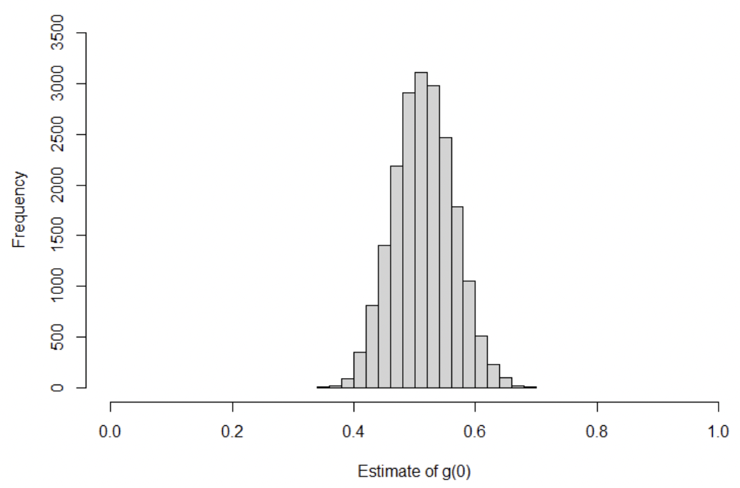
  • g(0) for the DAS data was included as an informed prior, assuming a beta distribution with shape parameters (47.6, 45.9) following data from Teilman et al. (2013) where the median estimate of porpoise availability (time spent at 0-2 m depth) was 0.58.
  • vp was to be estimated by the model with a Uniform prior between 0 and 0.003 (based on results from Jacobson et al., 2017).
  • n_l,d were the number of PPS observed between 0600 and 1800 summed over 4 days.
  • T_l,d was included as the summed number of seconds surveyed by the CPODs over the 4 days.
• Markov Chain Monte Carlo methods were used in the R-packages nimble (NIMBLE Development Team, 2023) and runjags (Denwood, 2016) to fit and evaluate the model. Four chains of 250,000 iterations with a burn-in period of 200,000 iterations was used, with a thinning rate of 10.
• Using the estimated vp values, density estimates could be derived from the PAM data. Daily PPS counts from the 1^st August to 1^st October 2010 were extracted to create a time series of daily absolute density estimates. Variances of the daily density estimates were estimated using the Delta method to combine all sources of uncertainty.
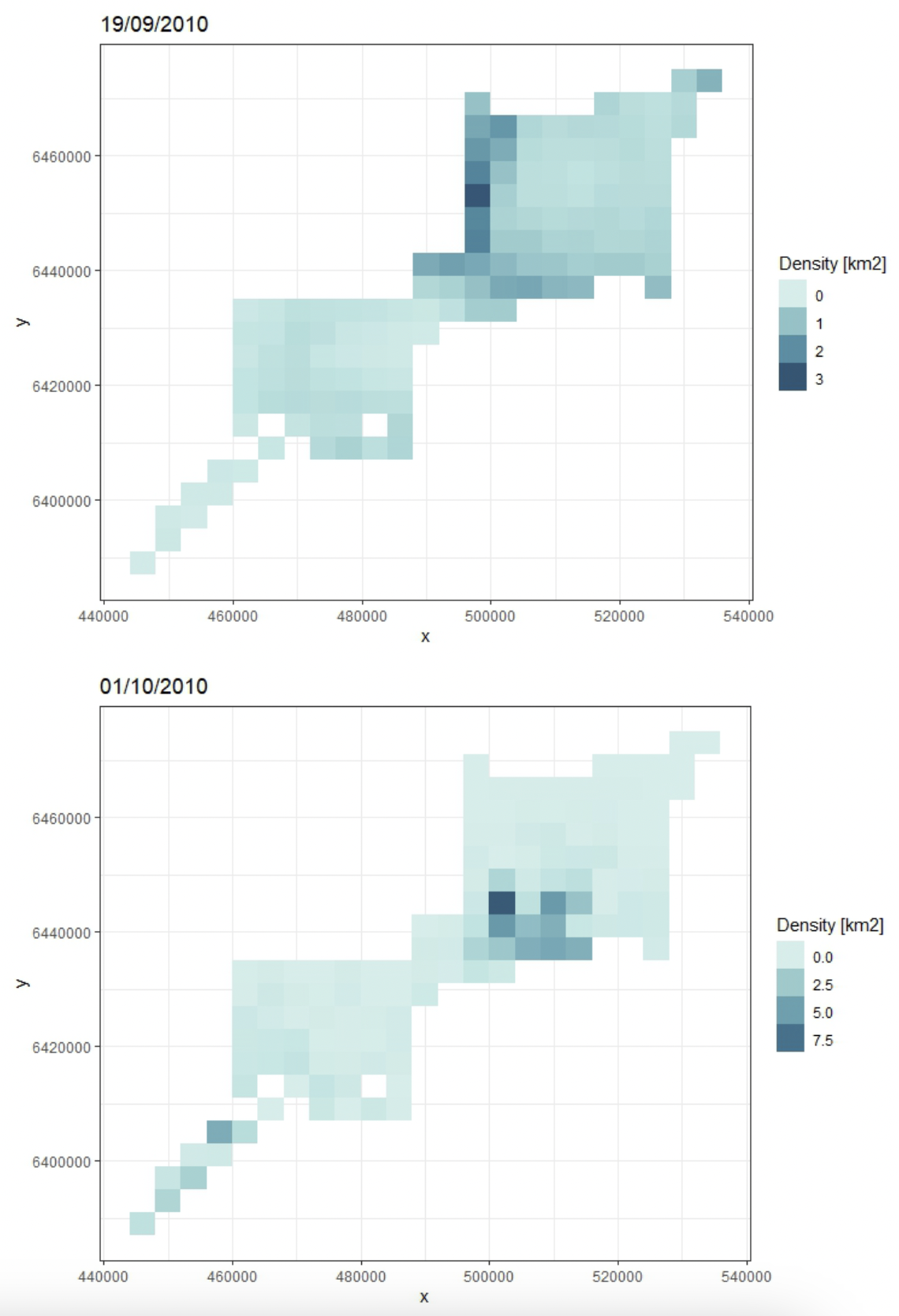
• Finally, a new absolute density surface was estimated from the resulting density estimates based on the PAM data. The same model fitting, model selection and model prediction approaches were used as for the spatial modelling based on DAS data only. If more than one CPOD overlapped with a given grid cell, a mean value of the devices was used as an input to the modelling. The same covariates as the DAS-only model were fitted to the resulting densities for one of the days when DAS was conducted (19 September) and to a day outside that period (01 October) to show the utility of the calibration method. A quasi-Poisson distribution was assumed for the response variable as the response variable was not count (as in case of DAS-based modelling) but density. Bootstrapping was used as described above for the DAS spatial models to estimate spatial modelling uncertainty around the generated density surfaces. Further bootstrapping routines would be required to include additional uncertainty from the vp estimation.

Results

Estimating density using DAS

Over the 4 days, a total of 2,155 km of completed DAS transect lines resulted in 97 observations of individual harbour porpoises. Specifically, 17, 11, 41, and 28 observations of individual porpoises were made on each of the separate survey days. The corresponding DAS-only absolute density estimate was 0.67 animals/km^-2 (95% confidence interval: 0.53 – 0.86 animals/km^-2).

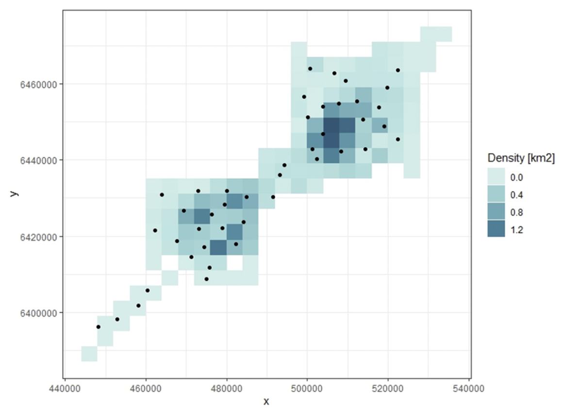
The best model fitted to the DAS data used a Tweedie distribution and included coordinates, depth and slope as natural cubic splines. The mean DAS-derived density across the whole prediction grid was 0.52 animals/km^-2. The DAS-derived densities assigned to the CPOD locations ranged between 0 and 2.0 animals/km^-2, with a mean of 0.57 animals/km^-2 (95% confidence interval: 0.43 – 0.95 animals/km^-2) (Fig 4). These estimates were comparable to those in Williamson et al. (2016).

Estimating density using DAS and PAM

CPOD data were available from 43 CPODs. Between 06:00 and 18:00, the mean number of PPS on the CPODs (summed across the four days of surveying) was 107, ranging between 0 and 613 PPS.

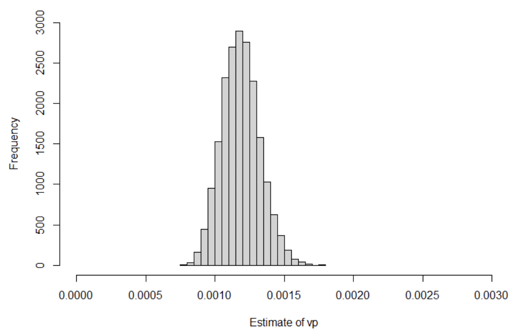
The model estimated the median value of vp to be 0.0012 (95% credible interval: 0.00094 – 0.0015) (Fig. 5). The estimate of g(0) was very similar to the assumed prior distribution; the median value was estimated to be 0.51 (95% credible interval: 0.42 – 0.61) (Fig. 6).

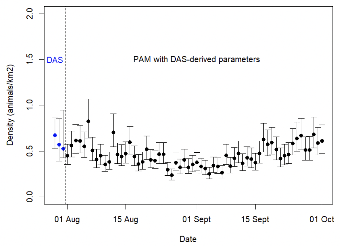
Using the estimates of vp and g(0), separate density estimates could be derived for each day from 1^st Aug – 1^st Oct 2010, including days where no DAS data were available. The median densities (averaged across all CPODs) for each day ranged between 0.24 and 0.83 animals/km^-2 (Fig. 7). The daily surfaces fitted using the calibrated PAM data showed differing daily patterns (Fig. 8).

Discussion

The case study implemented a Bayesian data integration method based on the methods in Jacobson et al. (2017). By estimating a parameter combining detection probability of harbour porpoise clicks and probability of clicking (vp), as well as g(0), PAM data could be converted to absolute density at a daily resolution, including days when the DAS data were not being collected (Figs 7 and 8). All daily estimates from the PAM data were on the same order of magnitude as the DAS-derived estimates (Fig 7). The method also accounts for uncertainty propagation (where included in the model) allowing confidence intervals to be estimated for all density estimates. In this analysis, uncertainty in g(0) and the DAS-derived estimates was included by incorporating these inputs as informed priors in the model.

A key aspect of this model is that the average estimates for vp and g(0) are assumed to be constant both over the period considered and over space (albeit with uncertainty). This is especially important for using the parameter estimates to estimate densities from the PAM data; a decision must be taken about how reasonable it is to use the estimates on days where there were no DAS surveys. The parameter of vp is a combination of CPOD EDA and the probability that a porpoise is vocally active in a 1-second time period. Due to changes in oceanographic conditions, it is possible that the EDA of a CPOD will change under differing ambient noise conditions, which may change seasonally. Therefore, despite the CPODs being deployed for several months, densities were only estimated between 01 Aug 10 and 01 Oct 10, given that the DAS surveys occurred in August and September, and assuming that conditions remained similar throughout this period. A next research step would be to alter the model to estimate vp for individual CPODs as suggested by Jacobson et al. (2017), and potentially as a function of date to more accurately predict vp for other dates, though more calibration DAS flights would likely be needed.

The average vocal behaviour of a porpoise is also assumed to remain constant over the survey time being considered (in this case 01 Aug – 01 Oct 2010). We do note in this study that seismic survey activity occurred during the data collection period and, if such activity altered harbour porpoise vocal behaviour, then the estimate of vp applied to days with seismic activity could be biased. Therefore, it is important to consider how representative the estimated parameters are of the wider dataset, especially when deciding which PAM data to apply the parameters to.

We also limited the CPOD data to daylight hours, to better match the DAS survey data. This means that our estimate of vp contains information about porpoise vocal behaviour specifically in daylight hours. However, we could readily include all CPOD data across all hours each day; the only assumption we would have to make is that the DAS-derived densities from daylight hours are applicable to hours of darkness as well. This may be reasonable to assume unless porpoises consistently migrated in or out of the survey area in hours of darkness. In that case, a more fine-scale study would be needed to understand potential diurnal changes in porpoise density and distribution, if such fine-scale changes needed to be understood for a given study (e.g., Williamson et al., 2022).

This case study focused on harbour porpoise using CPODs and DAS surveys. However, there is no reason why the same framework could not be implemented for other cetacean species, using different PAM instrumentation and even aerial surveys using human observers. However, the method is likely to be more successful for some species than others. Cetaceans with seasonal vocal behaviour (such as some baleen whales) may not make enough calls at a daily scale to calibrate effectively (the variability may be too high), but it is likely that the method will work well for other echolocating odontocetes, provided that the aerial surveys can provide robust estimates for calibration. Therefore, the calibration method may be a challenge for deep-diving odontocete species such as beaked whales, where visual-based estimates often have high uncertainty due to low sample sizes. Further, details of the method e.g., the specific acoustic unit of detection used for the PAM survey, will differ between species.

Finally, there are other data integration methods available as reviewed in Section 1. Therefore, a next research step would be to compare other reviewed methods with the calibration approach to assess the various strengths and limitations of the different methods. This would be an important step before recommending a standard approach to data integration.

Relevant code and data used for the case study are available on GitHub.