Harbour and grey seals: distribution maps

8. Appendices

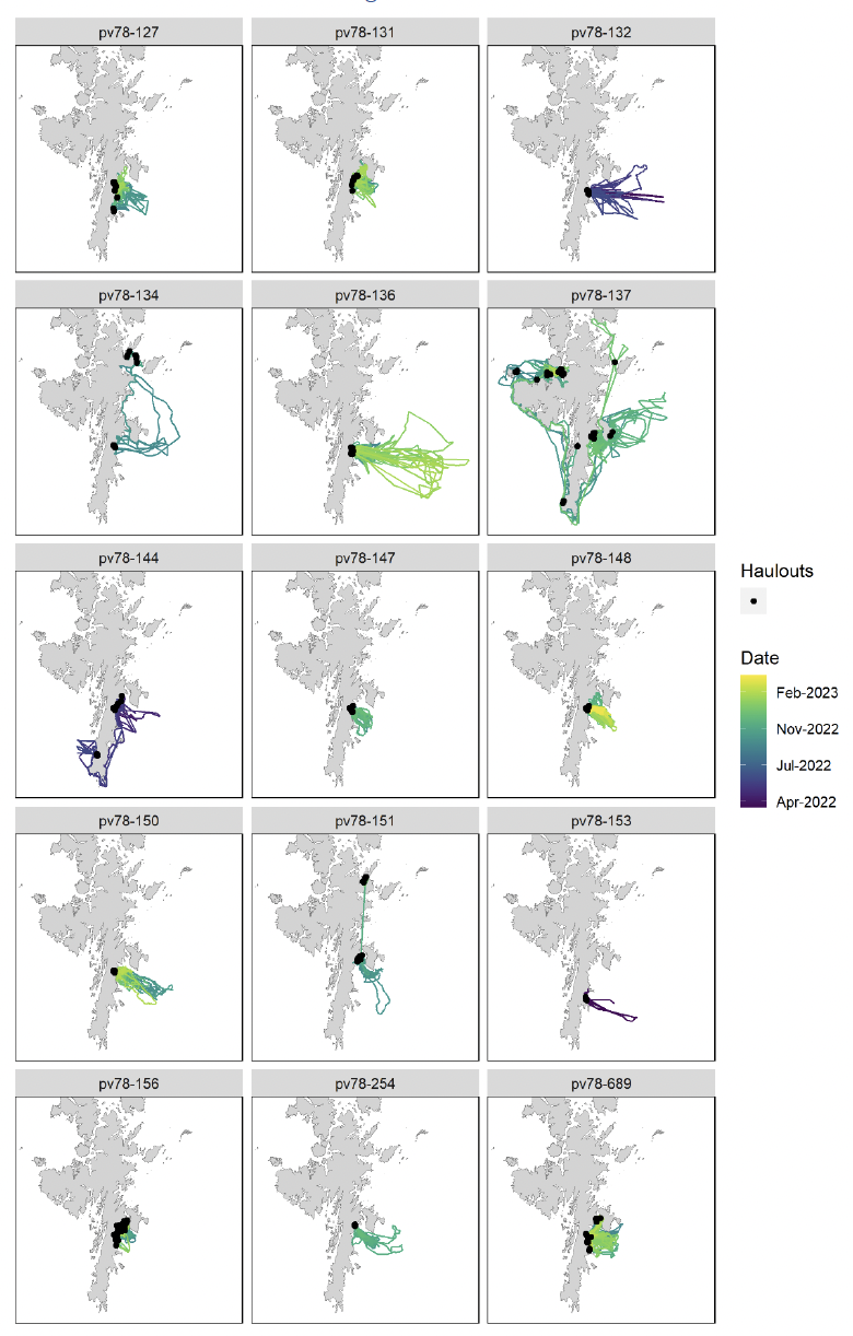
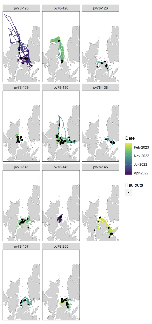
8.1. Shetland Harbour Seal Tracking Data

8.2. Habitat Preference Modelling Methods

8.2.1. Data Processing

Tracking data were first cleaned to remove erroneous location fixes and partitioned into trips using start and end haulout locations following the protocol outlined in Carter et al. (2022). Trips were assigned to different habitat preference regions based on the location of the haulout sites used before and after a trip, and trips that started in one region and finished in another were excluded. As per Carter et al. (2022), habitat preference regions were assigned based on regional differences in movement patterns, habitat composition and diet (see Fig. 4, main text).

Data from any trip initiated during the first week after tagging were excluded to remove any potential bias associated with altered behaviour resulting from capture. As per Carter et al. (2022), data were clipped to summer (May – August) for grey seals or autumn-winter-spring (September – May) for harbour seals to remove any locations during breeding and moult seasons. Locations were then interpolated to a constant 30-min time step, and any interpolated location with no observed GPS fix in the surrounding six hours was flagged as unreliable and excluded from the dataset. Each presence (interpolated location) was then matched to 30 control points which were randomly spaced within a trip-specific availability polygon, defined based on the maximum swimming distance (i.e., accounting for land barriers) travelled from a haulout of any individual in that species-region combination. The area beyond the continental shelf break (taken here as the 600 m isobath) was excluded from accessibility polygons since this is unlikely to represent viable habitat for seals (Carter et al., 2022). Environmental covariate values (see Section 8.2.2 below) were then extracted for all presences and control points. The ratio of control points to presences can have a dramatic effect on model inference if the availability sample does not effectively capture the composition of available habitat (Beyer et al., 2010). As per Carter et al. (2022) preliminary models were fitted with ratios between 1:1 and 1:30, and model coefficient values plotted to identify the ratio at which values stabilised. This analysis showed that a ratio of 1:30 was sufficient to adequately capture the available environment in all species-region combinations. For a more detailed account of data preparation protocols and the use-availability design, please see appendices in Carter et al., (2020).

8.2.2. Environmental Covariates

Environmental data from a range of data sources were extracted for every presence and control point, and included as explanatory covariates in the habitat preference models. Covariates were chosen on the basis of biological relevance to seals and/or their prey, or to control for the effects of accessibility on habitat selection. Firstly, distance to haulout (accounting for land barriers) was calculated and included to control for decreasing accessibility with increasing distance (Matthiopoulos, 2003). Distance to coast was also included since visual inspection of tracking data around Shetland revealed seals travelling far from the haulout but remaining very close to the coast. For example, a harbour seal was recorded 76 km from the haulout, but only 300 m from the coast. Coastline data were accessed from the European Environment Agency (EEA) Datahub.

Seabed geomorphology is known to influence the behaviour of some individual seals (Wyles et al., 2022). A dataset of geomorphological features for the Northeast Atlantic was generated from the freely available EMODnet harmonised gridded digital terrain model (DTM) for European sea regions (EMODnet Bathymetry, 2020). The DTM data were processed using the “r.geomorphon” extension for the Geographic Resources Analysis Support System (GRASS GIS) (Neteler & Mitasova, 2007) developed by Jasiewicz & Stepinski (2013), as described in Wyles et al. (2022). Seabed substrate type has also been shown to influence the habitat selection of harbour and grey seals in Scotland (Aarts et al., 2008; Carter et al., 2022), thus substrate type was extracted from the EMODnet Broad-Scale Habitat Map for Europe (EMODnet Seabed Habitats, 2021).

For grey seals, vertical water column stratification during summer has been shown to be an important predictor of habitat use in some regions (Carter et al., 2022). Summer mean potential energy anomaly (PEA) values were extracted from a data product developed under the Ocean Data Tool (ODaT) project (Jones, 2024). This covariate represents the amount of energy required in J/m³ to result in complete mixing of the water column under “typical” conditions for a given time of year. Thus, areas where the water column is fully mixed would have a PEA value of 0, and high values are associated with areas of strong water column stratification. This covariate was not included for harbour seals as there was little variation in PEA values experienced by the seals during the months coinciding with the tracking data.

As in Carter et al. (2022) “shelf” was included as a binary categorical term for grey seals hauling out in the Western Isles to account for the fact that many foraging trips were concentrated within 20 km of the shelf edge (600 m isobath). Bathymetric depth was included in preliminary models but was found to cause issues of high concurvity (assessed using the “performance” package (Lüdecke et al., 2021) in R (R Core Team, 2023)), and thus was excluded from further analyses. Retaining a covariate with high concurvity may result in over-estimation of model variance and masking of the effects of other covariates. All processing and extraction of environmental covariates was done using the “terra” (Hijmans, 2023) and “sf” (Pebesma & Bivand, 2023) packages in R.

8.2.3. Statistical Modelling Framework

For each species-region combination, control points and presences were modelled as a binary response term (0/1: available/used) as a function of the environmental covariates in a GAMM using the “bam” function in the “mgcv” package (Wood, 2017) in R. A binomial error family was specified with a logit link function. An individual seal identifier was included as a random intercept term using the “re” basis spline, allowing the modelled relationships to be estimated across individuals rather than data points, and ensuring that data-rich individuals did not unduly affect the results. Continuous covariates (distance to haulout, distance to coast and PEA) were modelled with a cubic regression spline with shrinkage, such that uninformative terms can be penalised to zero (Wood, 2017). To avoid over-fitting of smooth functions to the data, the number of knots (k) was limited to a maximum of five. Categorical covariates (geomorphology and substrate) were included both individually and in an interaction term.

Preliminary analysis revealed significant serial autocorrelation in model residuals for “used” data points. If ignored, this residual autocorrelation may lead to underestimation of model uncertainty. Examination of the partial autocorrelation function applied to residuals revealed that a first-order autoregressive (AR1) correlation structure would be appropriate. An AR1 structure was therefore applied with each trip treated as a separate time series. Each control point was also treated as a separate time series, such that no dependency was assumed between them, since they were randomly distributed in space. The correlation coefficient value ρ was determined by calculating the autocorrelation value of residuals for “used” points with residuals for “used” points at lag 1 for each trip for each seal. The median value across trips was then calculated for each seal, and the overall median of these seal-specific values was used as ρ in the final model. Model residuals were again examined after fitting to determine if the value of ρ was sufficiently high.

No model selection was undertaken, since the goal here was to find the best model for predicting distribution, rather than making biological inference about habitat selection. Thus, it was deemed better to retain all covariates rather than risk removing a potentially informative covariate, since non-informative terms that remained in the model would have little to no effect on the resulting distribution estimates.

8.2.4. Predicting At-Sea Distribution

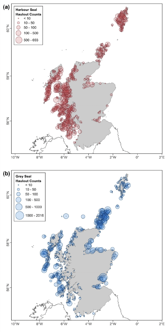
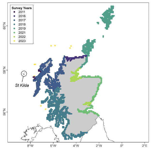
As in Carter et al. (2022), predictions of at-sea distribution (mean and associated lower and upper 95% confidence intervals) were generated on a 5 km x 5 km grid encompassing the marine area accessible to seals from all haulouts. Environmental data corresponding to the modelled covariates were first extracted for each cell in the prediction grid. Spatial predictions were then made emanating from each haulout site in Scotland with a non-zero count on the most recent survey (with the exception of the St Kilda archipelago, for which count data were not available; see Appendix Section 8.3 below), using the corresponding species-region model. Predictions were weighted by the relative area of sea in each cell (i.e., a coastal cell with 50% land cover would be weighted as 0.5), estimated using the EEA coastline dataset and the R package “extactextractr” (Baston, 2023). Raw predictions (on the logit scale) were exponentiated, then normalised (Manly et al., 2002). Haulout-specific prediction surfaces were then weighted by the number of individuals counted on the most recent survey, and summed into one multi-region surface per species. The multi-region surfaces were then normalised, such that the sum of values for all cells in the mean layer is 100, representing the percentage of the at-sea population predicted to be present in each cell (i.e., relative density). Cell-wise lower and upper 95% confidence intervals were generated using a posterior simulation approach (Carter et al., 2022; Wood, 2017).

8.3. Count Data